Unsurprisingly since essay 26 was a first cut at selective attention, it exposed a number of problems with both the neuroscience and the simulation model itself.
Specific give up
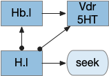
The current give up circuit is a global circuit, which doesn’t depend on the current stimulus. For this essay, the animal has two potential and because the give up is global, when the animal gives up, it gives up on both odors.
Global give-up circuit for olfactory seek. H.l lateral hypothalamus, Hb.l lateral habenula, Vdr dorsal raphe, 5HT serotonin.
An improvement would be a cue-specific give up capability. When the animal gives up on odor A, it should investigate odor B. Instead it gives up on both. I need to add some mechanism to create a cue-specific give up capability.
As a possible neural analog, the adenosine receptor can work as a local give-up circuit by integrating neural activity. Since adenosine is essentially a waste produce from neural activity, long activity will accumulate adenosine. The A1 adenosine receptor detects the adenosine and inhibits activity, since it’s a Gi receptor.
Olfactory complexity and attention
The essay’s odor model is extremely oversimplified, because odor receptors are feature detectors, not molecule receptors, and odors are combinations of molecules. Since a specific odor is a combination of features, P.bf (basal forebrain) can’t be a simple winner-take-all inhibitory circuit as implemented in this essay. Instead, attention needs to be a set of features that excludes the distractor odor’s features.
Olfactory gamma and beta
Although the essay treats the olfactory bulb data as direct signals, oscillations are a major feature of the olfactory bulb. Strong odors trigger gamma (40-100Hz) signals in Omt (mitral/tufted output cells), enhanced by ACh (acetylcholine) from P.bf. Feedback from O.pir (olfactory piriform cortex) triggers beta (15-30Hz) oscillations. In addition, interactions with breathing in mammals synchronized with theta (4-10Hz). Although, in the last case, since the simulation animal is aquatic, breathing isn’t an appropriate synchronizer.
Temporal gradient seek issues
Odor seeking in essay 26 uses temporal gradient descent modulated by head direction in Hb.m (medial habenula) and B.ip (interpeduncular nucleus). The animal combines its head direction with the temporal gradient to estimate the odor direction, and it saves the result as a goal vector. As the animal turns, it can improve the direct estimate. In the phototaxis example of essay 25, the saved goal vector direction helped with intermittent data, where it could remember the light location for a few seconds.
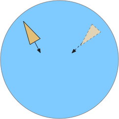
Problems with the current odor direction. A quick switch in location incorporates data from the old direction, leading to an incorrect estimate.
However, the system as implemented in the model is extremely limited. It can’t truly triangulate to locate the odor, but can only improve the single direction. In the diagram above, the animal can only select one of the two vectors as an estimate. It can’t combine the two into a better estimate of the center. Also, in the diagram, the earlier estimate is no longer useful because the animal has moved.
Now, the issue might be purely in the simulation. If B.ip and Vdr (dorsal raphe serotonin) are calculating this kind of estimate, it’s likely their computation is better than the current simulation.
The selection is a trade off where a stronger gradient is likely a better estimate, but if the animal moves too far from the earlier sample, the old direction is no longer relevant. Since the animal lacks the sophistication of an allocentric map to resolve the discrepancy, it discards the old value.
The current implementation decays the old estimate to allow newer estimates to overwrite it even if the later gradient is weaker. Essentially the memory is like a leaky integrator, as is appropriate for placing it in the serotonin neurons and/or associate glia with short term (5s) memory as in simple zebrafish motor memory [Dragomir et al 2020].
Bayesian updates
In a future essay, it might be interesting to explore this issue to see if a simple Bayesian system could be implemented in low-complexity circuits, where stronger data would update the current model more than the current model.
Self motion and gradient vectors
When the animal is turning, the running average no longer represents a straight line. For the gradient vector, the system assumes the recent average was measured along the current head direction, but turns violate this assumption. To avoid miscalculating gradient vectors, the animal should suppress measurement during turns.
Swimming and theta
The gradient seek issues above are compounded with swimming with a fixed head. Early vertebrates would have had a fixed head like sharks, meaning that each swimming stroke would move the head from side to side. That sideways movement would affect the odor gradient and head direction.
Inconsistent head vs body direction and odor measurement while swimming with a fixed head.
A simplistic fix would take an odor gradient sample only on each swim stroke, only reporting at the stroke end for consistency and to average from the beginning of the stroke to the end. That solution would give a consistent measurement in a reasonably consistent direction, as opposed to sampling randomly in a cycle.
Log encoding vs linear encoding
For simplicity, I’e used linear encoding for signals in the essays, because the basic functional architecture remains the same, and the simulation isn’t precise enough to need more complexity. But for odors, the dynamic range between a single molecule detection and an overpowering odor doesn’t scale well with a linear representation.
In particular, the odor weight from the simple distance gradient, together with above mentioned temporal gradient issues might be better modeled with a log signal. Basically, the issue I raised above with gradient vector sampling might be more tractable with a different encoding, and log encoding might make the actual neural circuit less finicky than the current linear model.
Seek mode switching
The essay’s simulation lacks a specific mode switching circuit. In vertebrates the peptide core (hypothalamus, PAG, B.pb area) switches action modes from roaming to seek to eating to rest and sleep. These modes are motivated and depend on internal needs and scheduling impulses programmed by evolution.
Although the previous essays have focused on bilateral locomotion in the style of Braitenberg machines, the chimaera brain hypothesis [Tosches and Adrendt 2013] suggests a distinct apical form of locomotion. The chimaera brain hypothesis suggests that bilaterian brains are the merger of an apical nervous system from the ancestral zooplankton larva state and a blastoporal (bilateral) nervous system from paired muscles along the spinal cord. The apical area contains unpaired light and chemical sensors and the blastoporal area contains bilateral, topographic somatic sense like touch. Apical navigation require a temporal gradient, calculated by sequential sampling because the apical senses are non-directional.
Apical unpaired light sensors and bilateral paired touch sensors in the chimaera brain.
The essays’ simulation scenario is a temporal phototaxis based on the real-time place preference (RTPP) experiments of [Chen et al 2014], where a zebrafish stayed inside a virtual light circle, avoiding surrounding dark area. Temporal phototaxis is gradient-based locomotion, heading toward light and away from darkness by comparing light samples at different times.
Chimaera locomotor
The vertebrate paired eye and paired olfaction are late vertebrate developments. The pre-vertebrate animal amphioxus has only a single frontal eye. Since pre-paired sense animals needed to navigate toward opportunities and away from threats, it’s conceivable that apical random-walk navigation developed before visual navigation.
Dual navigation system based on both temporal gradient-based random walks and bilateral spatial gradient navigation.
Apical gradient
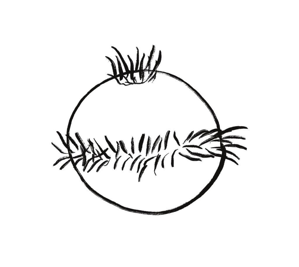
The apical area contains undirected light and chemical sensors. The apical area is based on the zooplankton larval state as shown below, while the bilateral area is based on bilateral worm-like adults structured like the spinal cord of paired muscles and neurons.
Apical zooplankton larva. Note the single sensor on top.
Apical navigation requires following a temporal gradient, calculated by sequential sampling. While bilateral areas can compare left and right senses to calculate a spatial gradient, the single apical sense is restricted to a temporal gradient.
Bacteria tumble and run
Even simple bacteria can follow gradients using a directed random walk strategy called tumble and run [Segall et al 1986]. The bacteria’s flagella have two modes: tumble, turning without moving, and run, moving forward without turning. By alternating tumble with run, the bacteria can search with a random walk. By extending the run phase when the gradient improves, the bacteria can move toward the target.
Importantly, a temporal gradient calculation needs some sort of memory, accumulator or integrator to compare the current value to recent values. In bacteria, tis accumulator is an internal chemical quantity.
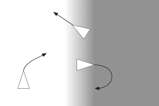
Different turning behavior depending on the gradient. Sharp turns moving into darkness and straight movement into light.
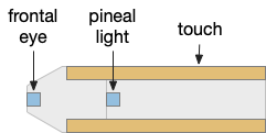
Apical and bilateral sensors
Amphioxus is a pre-vertebrate chordate that’s studied to understand vertebrate evolution. Amphioxus does not have a paired eye, instead it has a single frontal eye that amphioxus uses to orient vertically, and also a pineal-like photoreceptor [Lacalli 2020].
The pineal region is near the vertebrate habenula. Amphioxus does not have a habenula, but it does have a nearby motor control neuron, LPN3, with similar genetic markers [Bozzo et al 2023]. Modern vertebrate medial habenula receives undirected light input from the retina, but it seems plausible that an early habenula used the pineal photosensor because both are part of the same epithalamus complex, and only later connected to the newly-paired retina when it developed.
Multiple apical regions
Before diving into the vertebrate areas for apical locomotion, I need to explain why widespread areas can all be apical, including midbrain and hindbrain areas. Vertebrates had two rounds of whole genome duplication [Dehal and Moore 2005], which gives an easy evolutionary opportunity for four apical areas from the genome duplication, in addition to other possible duplications. The xenobot experiments [Blackiston et al 2023] shows that biology can mix multiple copies like the split apical area into a coherent animal: development can be flexible.
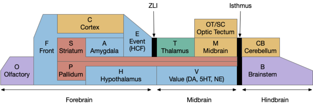
Functional vertebrate brain model showing apical areas as marked by fgf8 development transcription factor.
The diagram above is a functional representation of the vertebrate brain with possible apical areas highlighted in blue. Fgf8 is a development growth factor associated with the apical area [Marlow et al 2014]. The four (or five) possible apical area are as follows:
Prefrontal cortex and olfactory bulb.
The caudal isthmus area (r1) at the midbrain-hindbrain boundary, including cerebellum (CB), interpeduncular nucleus (M.ip), midbrain locomotor (MLR, M.ppt, M.ldt), head direction (B.dtg), parabrachial (B.pb), and part of the substantia nigra (Snr).
Habenula (Hb) and pre-thalamic eminence area (P.em) near ZLI. Also, between the septum-diagonal band (P.msdb) and preoptic area (Poa) near the optic (retina) region (R).
The mammilary and supramammilary area of the hypothalamus (H.mb and H.sum).
I’ve listed four regions instead of the five blue areas because the Hb-P.em-P.msdb area are physical closer than the diagram suggests, are split more by the alar/basal division than distance, and is complicated by distortions from the paired optic region.
This essay uses functions from the r1 isthmus area (M.ip and MLR.α / M.ldt), and from the habenula / retinal area (Hb.m, P.em, pineal, and retina). The logic behind their connectivity is a function split-and-pull like taffy or continental drift from a single pre-duplication area, for example, the isthmus apical area duplicating from an original pre-hypothalamus / retinal apical area.
As a note, the supramammilary area (H.sum) is highly connected with the area in this essay, but I’m postponing exploring its functionality for now.
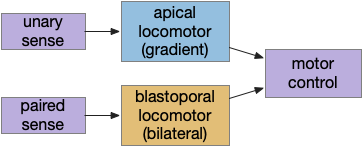
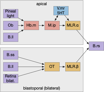
Vertebrate apical and bilateral locomotor
Previously the essays used the bilateral locomotor path, going through the Vta (posterior tuberculum), tectum (OT), and midbrain locomotive region (MLR). The apical path runs through the medial habenula (Hb.m) and the interpeduncular nucleus (M.ip) before reaching the motor neurons.
Bilateral and apical locomotive paths. B.ll lateral line, B.rs reticulospinal motor neurons, B.ss somatosensory, Hb.m medial habenula, M.ip interpeduncular nucleus, MLR midbrain locomotive region, OT optic tectum, V.mr median raphe, 5HT serotonin.
The lamprey’s Hb.m supports locomotion for light, odor, and the lateral line [Stephenson-Jones et al 2012]. The lateral line is an aquatic sense for water flow, which allows fish to sense nearby objects. Although the exact functional division of phototaxis isn’t known, Hb.m, M.ip and the serotonin raphe nuclei (V.mr – 5HT) are all required [Cheng et al 2016].
For the essay’s simulation, I’m asking the integration and running average to the V.mr and 5HT, but this is something of a guess, because phototaxis integration hasn’t been measured. In the essay’s model, M.ip translates the light data and 5HT average into a gradient and into action.
Phototaxis actions
When zebrafish enter darkness from light, they immediately produce a large turn (O-bend) and start an area restricted search (ARS) [Fernandes et al 2012]. Later turns are smaller [Chen and Engert 2014].
For the essay, phototaxis gradient modifies the standard random walk. When entering darkness, M.ip increases the turn angle. When entering light, M.ip increases forward movement, extending the run.
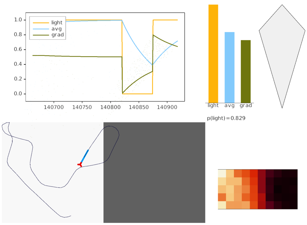
Essay simulation showing the animal returning to light from darkness. The graph shows the gradient change when crossing the darkness boundary.
The above screenshot shows the animal crossing into darkness and returning to light. In the graph, “light” is the current photosensor value, “avg” is the running average measured by serotonin neurons, and “grad” is the different between the two. A gradient drop triggers high angle turns. A gradient rise triggers straight movement.
As the heat map in the right shows, this simple system produces real-time place avoidance (RTPA) of darkness. Since the system has no learning, there’s no conditioned place aversion (CPA).
Prethalamic eminence
The full phototaxis circuit in vertebrates is a bit more complicated because light input does through an intermediate area called the pre-thalamic eminence (P.em), which is between the habenula, hypothalamus and thalamus, and it one of the apical areas. Although P.em is not cortical, it provides neurons necessary for cortical development (Cajal-Retzius neurons for L1 patterning) [Marin-Padilla 2015] and neurons for habenula input, the habenula-projecting pallidum (P.hb) [Stephenson-Jones 2016].
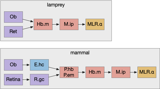
Apical navigation paths, simplified in lamprey and extended in mammals. E.hc hippocampus, Hb.m medial habenula, M.ip interpeduncular nucleus, MLR midbrain locomotive region, Ob olfactory bulb, P.em pre-thalamic eminence, P.hb habenula projecting pallidum, R.gc retina ganglion cells.
Retina input goes through P.em to Hb.m for phototaxis. Interestingly, the main input for Hb.m in mammals is via cells that migrate from P.em and become the posterior septum (P.ps) [Watanabe et al 2018], which receives almost all of its input from the hippocampus (E.hc). If the hippocampus is an odor-processing system, then the olfactory bulb (Ob) to E.hc to Hb.m path is a chemotaxis path matching the retina’s phototaxis path.
Note that the olfactory placed develops from the lens placed and is differentiated by fgf8 [Bailey et al 2006]. So, it’s pleasing that the similar olfactory and hippocampal paths to Hb.m is a are chemotaxis and phototaxis paths split from a common ancestor.
Speculation
Although the lateral and medial habenula are chemically, connectional, and developmentally distinct, their broad similarity is interesting. If the medial habenula supports direct, concrete sensory navigation by gradient descent, perhaps the medial habenula supports more abstract value-based navigation for more abstract goals.