The essay 16 simulation is a foraging slug that follows odors to food, which must give-up on an odor when the odor plume doesn’t have food. Foraging researchers treat the give-up time as a measurable value, in optimal foraging in the context of the marginal value theorem (MVT), which tells when an animal should give up [Charnov 1976]. This post is a somewhat disorganized collection of issues related to implementing the internal state needed for give up time.
Giving up on an odor
The odor-following task finds food by following a promising odor. A naive implementation with a Braitenberg vehicle circuit [Braitenberg 1984], as early evolution might have tried, has the fatal flaw that the animal can’t give up on an odor. The circuit always approaches the odor.
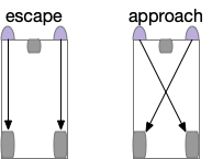
Since early evolution requires simplicity, a simple solution is adding a timer, possibly habituation but possibly a non-habituation timer. For example, a synapse LTD (long term depression) might ignore the sensor after some time. Or an explicit timer might trigger an inhibition state.
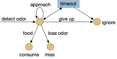
In the diagram, the beige nodes are stateless stimulus-response transitions. The blue area is internal state required to implement the timers. This post is loosely centered around exploring the state for give-up timing.
Fruit fly mushroom body neurons
Consider a sub-circuit of the mushroom body, focusing on the Kenyon cell (KC) to mushroom body output neuron (MBON) synapses, and the dopamine neuron (DAN) that modulates it. For simplicity, I’m ignoring the KC fanout/fanin and ignoring the habituation layer between odor sensors and the KC, as if the animal was an ancestral Precambrian animal.
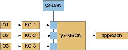
Give-up timing might be implemented either in the synapses in blue between the KC and MBON, or potentially in circuits feeding into the DAN. The blue synapses can depress over time (LTD) when receiving odor input [Berry et al. 2018], with a time interval on the order of 10-20 minutes. Alternatively, the timeout might occur in circuitry before the DAN and use dopamine to signal giving up.
In mammals, the second option involving a dopamine spike might signal a give-up time. Although the reward-prediction error (RPE) in the Vta (ventral tegmental area) is typically interpreted as a reinforcement-learning signal, it could also signal a give-up time.
Mammalian analogy
In mammals, a give-up signal might be a combination of some or all of several neurotransmitters: dopamine (DA), serotonin (5HT), acetylcholine (ACh), and possibly norepinephrine (NE).
Dopamine has a characteristic phasic dip when the animal decides no reward will come. Many researchers consider this no-reward dip to be a reward-prediction error (RPE) in the sense of reinforcement learning [Schultz 1997].
One of the many serotonin functions appears patience-related [Lottem et al. 2018], [Miyazaki et al. 2014]. Serotonin ramps while the animal is persevering at the task and rapidly drops when the animal gives. Serotonin is also required for reversal learning, although this may be unrelated.
Acetylcholine (ACh) is required for task switching. Since giving-up is a component of task switching, ACh likely plays some role in the circuit.
[Aston-Jones and Cohen 2005] suggest a related role for norepinephrine for patience, impatience and decision making.
On the one hand, having essentially all the important modulatory neurotransmitters involved in this problem doesn’t give a simple answer. On the other hand, the involvement of all of them in give-up timing may be an indication of how much neural circuitry is devoted to this problem.
Mammalian RPE circuitry
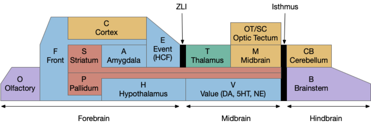
The following is a partial(!) diagram for the mammalian patience/failure learning circuit, assuming the RPE signal detected in DA/Vta is related to give-up time. The skeleton of the circuit is highly conserved: almost all of it exists in all vertebrates, with the possible exception ofr the cortical areas F.vm (ventromedial prefrontal cortex) and C.sma (supplemental motor area). For simplicity, the diagram doesn’t include the ACh (V.ldt/V.ppt) and NE (V.lc) circuits. The circuit’s center is the lateral habenula, which is associated with a non-reward failure signal.
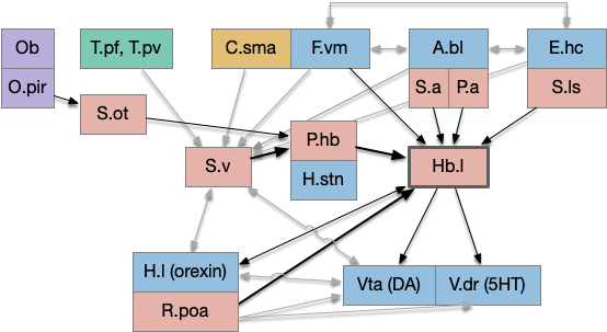
Key: T.pf (parafascicular thalamus), T.pv (paraventricular thalamus), C.sma (supplementary motor area cortex), F.vm (ventromedial prefrontal cortex), A.bl (basolateral amygdala), E.hc (hippocampus), Ob (olfactory bulb), O.pir (piriform cortex), S.v (ventral striatum/nucleus accumbens), S.a (central amygdala), S.ls (lateral septum), S.ot (olfactory tubercle), P.hb (habenula-projecting pallidum), P.a (bed nucleus of the stria terminalis), Hb.l (lateral habenula), H.l (lateral hypothalamus), H.stn (sub thalamic nucleus), Poa (preoptic area), Vta (ventral tegmental area), V.dr (dorsal raphe), DA (dopamine), 5HT (serotonin). Blue – limbic, Red – striatal/pallidal. Beige – cortical. Green – thalamus.
Some observations, without going into too much detail. First, the hypothalamus and preoptic area is heavily involved in the circuit, which suggests its centrality and possibly primitive origin. Second, in mammals the patience/give-up circuit has access to many sophisticated timing and accumulator circuits, including C.sma, F.ofc (orbital frontal cortex), as well as value estimators like A.bl and context from episodic memory from E.hc (hippocampus.) This, essentially all of the limbic system projects to Hb.l (lateral habenula), a key node in the circuit.
Although the olfactory path (Ob to O.pir to S.ot to P.hb to Hb.l) is the most directly comparable to the fruit fly mushroom body, it’s almost certainly convergent evolution instead of a direct relation.
The most important point of this diagram is to show that mammalian give-up timing and RPE is so much more complex than the fruit fly, that results from mammalian studies don’t give much information for the fruit fly, although the reverse is certainly possible.
Reward prediction error (RPE)
Reward prediction error (RPE) itself is technically just an encoding of a reward result. A reward signal could either represent the reward directly or as a difference from a reference reward, for example the average reward. Computational reinforcement learning (RL) calls this signal RPE because RL is focused on the prediction not the signal. But an alternative perspective from the marginal value theorem (MVT) of foraging theory [Charnov 1976], suggests the animal use the RPE signal to decide when to give up.
The MVT suggests that an animal should give up on a patch when the current reward rate is lower than the average reward rate in the environment. If the RPE’s comparison reward is the average reward, then a positive RPE suggests the animal should stay in the current patch, and a negative RPE says the animal should consider giving up.
In mammals, [Montague et al. 1996] propose that RPE is used like computational reinforcement learning, specifically temporal difference (TD) learning, partly because they argue that TD can handle interval timing, which is related to the give up time that I need. However, TD’s timing representation requires a big increase in complexity.
Computational models
To see where the complexity of time comes from, let’s step back and consider computational models used by both RL and the Turing machine. While the Turing machine might seem to formal here, I think it’s useful to explore using a formal model for practical designs.
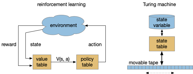
Both models above abstract the program into stateless transition tables. RL uses an intermediate value function followed by a policy table [Sutton and Barto 2018]. The Turing state is either in the current state variable (basically an integer) and the infinite tape. RL exports its entire state to the environment, making no distinction between internal state like a give-up timer and the external environment. Note the strong contrast with a neural model where every synapse can hold short-term or long-term state.
Unlike the Turing machine, the RL machine diagram is a simplification because researchers do explore beyond the static tabular model, such as using deep-learning representations for the functions. The TD algorithm itself doesn’t follow the model strictly because it updates the value and policy tables dynamically, which can create memory-like effects early in training.
The larger issue in this post’s topic is the representation of time. Both reinforcement learning and the Turing machine represent time as state transitions with a discrete ticking time clock. An interval timer or give-up timer is represented by states for each tick in the countdown.
State machine timeout
The give-up timeout is an illustration of the difference between neural circuits and state machines. In neural circuits, a single synapse can support a timeout using LTD (or STD) with biochemical processes decreasing synapse strength over time. In the fruit fly KC to MBON synapse, the timescale is on the order of minus (“interval” timing), but neural timers can implement many timescales from fractions of seconds to hours in a day (circadian).
State machines can implement timeouts as states and state transitions. Since state machines are clock based (tick-based), each transition occurs on a discrete, integral tick. For example, a timeout might look like the following diagram:
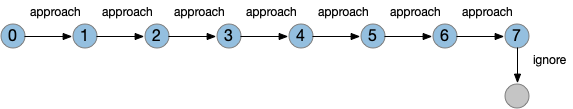
This state isn’t a counter variable, it’s a tiny part of a state machine transition table. State machine complexity explodes with each added capability. If this timeout part of the state machine is 4 bits representing 9 states, and another mostly-independent part of the state machine has another 4 bits with 10 state, the total state machine would need 8 bits with 90-ish states, depending on the interactions between the two components because a state machine is one big table. So, while a Turing machine can theoretically implement any computation, in practice only relatively small state machines are usable.
Searle’s Chinese room
The tabular nature of state machines raises the philosophical thought experiment of Searle’s Chinese room, as an argument against computer understanding.
Searle’s Chinese room is a philosophical argument against any computational implementation of meaningful cognition. Searle imagines a person who doesn’t understand Chinese in a huge library with lookup books containing every response to every possible Chinese conversation. When the person receives a message, they find the corresponding phrase in one of the books and writes the proper response. So, the person in the Chinese room holds a conversation in Chinese without understanding a single word.
For clarity, the room’s lookup function is for the entire conversation until the last sentence, not just a sentence to sentence lookup. Essentially it’s like the input the attention/transformer deep learning as use in something like ChatGPT (with a difference that ChatGPT is non-tabular.) Because the input includes the conversational context, it can handle contextual continuity in the conversation.
The intuition behind the Chinese room is interesting because it’s an intuition against tabular state-transition systems like state machines, the Turing machine, and the reinforcement learning machine above. Searle’s intuition is basically since computer systems are all Turing computable, and Turing machines are tabular, but tabular lookup is an absurd notion of understanding Chinese (table intuition), therefore computers systems can never understand conversation. “The same arguments [Chinese room] would apply to … any Turing machine simulation of human mental processes.” [Searle 1980].
Temporal difference learning
TD learning can represent timeouts, as used in [Montague et al. 1996] to argue for TD as a model for the striatum, but this model doesn’t work at all for the fruit fly because each time step represents a new state, and therefore needs a new parameter for the value function. Since the fruit fly mushroom body only has 24 neurons, it’s implausible for each neuron to represent a new time step. Since the mammalian striatum is much larger (millions of neurons), it can encode many more values, but the low information rate from RPE (less than 1Hz), makes learning difficult.
These difficulties don’t mean TD is entirely wrong, or that some ideas from TD don’t apply to the striatum, but it does mean that a naive model of TD of the striatum might have trouble working at any significant scale.
State in VLSI circuits
Although possibly a digression, I think it’s interesting to compare state in VLSI circuits (microprocessors) to both neurons, and the reinforcement learning machine and Turing machine. In some ways, state in VLSI resembles neurons more than it does formal computing models.
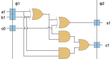
The φ1 and φ2 are clock signals needed together with the latch state to make the system work. The clocks and latches act like gates in an airlock or a water lock on a river. In a water lock only one gate is open at a time to prevent the water from rushing through. In the VLSI circuit, only one latch phase is active at a time to keep the logic bigs from mixing togethers. Some neuroscience proposals like [Hasselmo and Eichenbaum 2005] have a similar architecture for the hippocampus (E.hc) for similar reasons (keeping memory retrieval from mixing up memory encoding.)
In a synapse the slower signals like NMDA, plateau potentials, and modulating neurotransmitters and neuropeptides have latch-like properties because their activation is slower, integrative, and more stable compared to the fast neurotransmitters. In that sense, the slower transmission is a state element (or a memory element). If memory is a hierarchy of increasing durations, these slower signals are at the bottom, but they are nevertheless a form of memory.
The point of this digression is to illustrate that formal machine state models is unusual and possibly unnatural, even when describing electronic circuits. That’s not to say that those models are useless. In fact, they’re very helpful for mental models at the smaller scales, but in larger implementations, the complexity of the necessary state machines limits their value as an architectural model.
Conclusion
This post is mostly a collection of trying to understand why the RPE model bothers me as unworkable, not a complete argument. As mentioned above, I have no issues with a reward signal relative to a predicted reward, or using that differential signal for memory and learning. Both seem quite plausible. What doesn’t work for me is the jump to particular reinforcement learning models like temporal difference, adding external signals like SCS, and without taking into account the complexities and difficulties of truly implementing reinforcement learning. This post tries to explain some of the reasons for that skepticism.
References
Aston-Jones, Gary, and Jonathan D. Cohen. An integrative theory of locus coeruleus-norepinephrine function: adaptive gain and optimal performance. Annu. Rev. Neurosci. 28 (2005): 403-450.
Berry, Jacob A., et al. Dopamine is required for learning and forgetting in Drosophila. Neuron 74.3 (2012): 530-542.
Braitenberg, V. (1984). Vehicles: Experiments in synthetic psychology. Cambridge, MA: MIT Press. “Vehicles – the MIT Press”
Charnov, Eric L. “Optimal foraging, the marginal value theorem.” Theoretical population biology 9.2 (1976): 129-136.
Hasselmo ME, Eichenbaum H. Hippocampal mechanisms for the context-dependent retrieval of episodes. Neural Netw. 2005 Nov;18(9):1172-90.
Lottem, Eran, et al. Activation of serotonin neurons promotes active persistence in a probabilistic foraging task. Nature communications 9.1 (2018): 1000.
Miyazaki, Kayoko W., et al. Optogenetic activation of dorsal raphe serotonin neurons enhances patience for future rewards. Current Biology 24.17 (2014): 2033-2040.
Montague, P. Read, Peter Dayan, and Terrence J. Sejnowski. A framework for mesencephalic dopamine systems based on predictive Hebbian learning. Journal of neuroscience 16.5 (1996): 1936-1947.
Schultz, Wolfram. Dopamine neurons and their role in reward mechanisms. Current opinion in neurobiology 7.2 (1997): 191-197.
Searle, John (1980), Minds, Brains and Programs, Behavioral and Brain Sciences, 3 (3): 417–457,
Sutton, R. S., & Barto, A. G. (2018). Reinforcement learning: An introduction. MIT press.